Difference between revisions of "Examples/2D/souto etal 2012 standingwave"

Revision as of 11:14, 25 April 2015

Introduction

In this examples we are reproducing the simulation of the standing wave carried out by Souto et all (2012) ^[1].

The standing wave is defined on top of an infinite periodic fluid domain composed by rectangular subdomains of dimensions ${\displaystyle L\times H}$ , with ${\displaystyle L=2H}$ . In such domain a wave with length ${\displaystyle\lambda=L}$ (i.e. the wave number is ${\displaystyle k=2\pi/L}$ ) and amplitude ${\displaystyle A}$ is imposed. Denoting the ratio ${\displaystyle 2A/H}$ by ${\displaystyle\varepsilon}$ the following velocity potential can be considered:

${\displaystyle\phi\left(x,y,t\right)=\phi_{0}\left(x,y\right)\,\cos(\omega t),}$

${\displaystyle\phi_{0}\left(x,y\right)=-\varepsilon{\frac{H\,g}{2\omega}}{\frac{\cosh\left(k\left(y+H\right)\right)}{\cosh\left(kH\right)}}\cos\left(kx\right),}$

valid for small values of ${\displaystyle\varepsilon}$ . In previous equations ${\displaystyle\omega}$ is the angular frequency given by the dispersion relation of gravity waves: ${\displaystyle\omega^{2}=g\,k\tanh\left(k\,H\right)}$ , and ${\displaystyle y=0}$ corresponds to the flat free surface (In Fig. 13 of Souto et all (2012)^[1] it is wrong described)

Therefore the velocity field can be computed as ${\displaystyle{\mathbf{u}}\left(x,y,t\right)=\nabla\phi\left(x,y,t\right)}$ . It should be noticed that for ${\displaystyle t=0}$ a flat free surface is obtained.

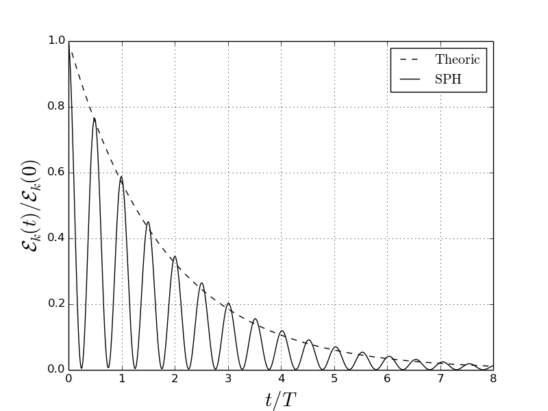
With such velocity potential, for a viscous fluid, it is possible to get an analytical solution for the kinetic energy decay^[2]:

${\displaystyle{\mathcal{E}}_{k}\left(t\right)=\varepsilon^{2}g{\frac{LH^{2}}{32}}e^{{-4\nu k^{2}t}}\left(1+\cos\left(2\omega t\right)\right),}$

where the kinematic viscosity can be computed from the Reynolds number:

${\displaystyle\nu={\frac{\mu}{\rho}}={\frac{H{\sqrt{gH}}}{{\mathcal{Re}}}}.}$

In our simulation ${\displaystyle g=1}$ , ${\displaystyle L=1}$ , ${\displaystyle\varepsilon=0.1}$ , ${\displaystyle\rho=1}$ and ${\displaystyle H/\Delta x=100}$ , where ${\displaystyle\Delta x}$ is the initial distance between the particles.

Setting up the simulation

In AQUAgpusph the examples are generated on top of template archives, which are read and modified by the Python Script Create.py, such that they can be ran from an arbitrary folder, and modified just touching such Create.py script.

You can run the prebuilt version of the example right after compiling AQUAgpusph:

cd examples/2D/souto_etal_2012_standingwave
./run.sh --run

Also you can plot the result in real time opening a new terminal (in the same place) and typing:

./run.sh --plot e

Resulting kinetic energy compared with the analytically computed.

However we are interested into setup the case from scratch, assuming that we are running it in the same folder we are creating the input files.

Presets

We are using a number of AQUAgpusph presets:

• cfd.xml: Should preset should be the first included for fluid dynamics problems.
• domain.xml: Even though in this problem it is not expected to get particles running away from the domain, it is strongly recommended to ever set a computational domain.
• energy.xml and energy.report.xml: In this problem the main result is the kinetic energy evolution along the time, so we ask to compute and print it to a file.
• timing.report.xml and performance.report.xml: Useful to profile the execution.
• symmetry.xml: To can impose symmetric boundary conditions.

To load all these presets (except symmetry.xml one, which we are managing later) we can create a file called Presets.xml, with the following content:

<?xml version="1.0" ?>
<sphInput>
    <Include file="/usr/share/aquagpusph/resources/Presets/cfd.xml" />
    <Include file="/usr/share/aquagpusph/resources/Presets/domain.xml" />
    <Include file="/usr/share/aquagpusph/resources/Presets/energy.xml" />
    <Include file="/usr/share/aquagpusph/resources/Presets/timing.report.xml" />
    <Include file="/usr/share/aquagpusph/resources/Presets/performance.report.xml" />
    <Include file="/usr/share/aquagpusph/resources/Presets/energy.report.xml" />
</sphInput>

Replacing /usr/share/aquagpusph by the AQUAgpusph folder.

Settings

References

1. ↑ ^{1.0 1.1} Antonio Souto-Iglesias, Fabricio Macià, Leo M. González, Jose L. Cercos-Pita. On the consistency of MPS. Computer Physics Communications, 2012
2. ↑ J. Lighthill. Waves in Fluids. Cambridge University Press, 2001